Visualize the results

Let’s consider a Geodesic object that has been integrated by following the procedures shown in the previous tutorials (see Integrate a geodesic in PyGRO).

For example, let’s consider the following geodesic in the Schwarzschild space-time:

geo = pygro.Geodesic("time-like", geo_engine)
geo.set_starting_point(0, 175, np.pi/2, 0)
geo.set_starting_4velocity(u1 = 0, u2 = 0, u3 = 2e-4)
geo_engine.integrate(geo, 50000, 1)

We want to visualize the results of the integration.

First of all we can access the exit status of the geodesic

print(geo.exit)

which is assigned by the GeodesicEngine object. In this case we obtain

>>> 'done'

signaling that the integration has been carried on for the entire interval of proper time indicated in the integrate() method. If a StoppingCriterion has been met the exit status of the Geodesic will correspond to the exit message of the criterion that stopped the integration (see Integrate a geodesic in PyGRO).

Once the geodesic has been integrated, the properties Geodesic.tau, Geodesic.x, and Geodesic.u will be filled with the arrays of proper times, integrated space-time cooridinates and components of the 4-velocity along the geodesic, respectively.

We can access them and plot them directly, by doing for example (using Matplotlib)

import matplotlib.pyplot as plt

fig, ax = plt.subplots()

ax.plot(geo.tau, geo.x[:,1])

ax.set_xlabel(r"$\tau$ ($M$)")
ax.set_ylabel(r"$r$ ($M$)")

which outputs

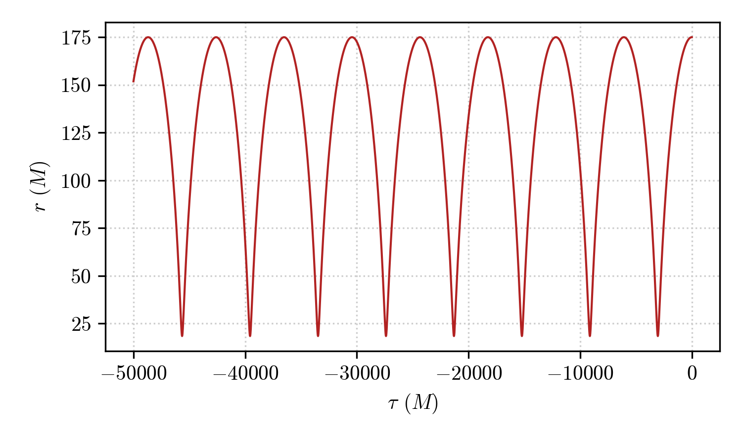
showing the radial component (geo.x[:,1]) as a function of the proper time (geo.tau).

We can do the same with the other components, or with any component of the 4-velocity. For example, one can plot the 0-th component of the integrated geodesic (in our case \(\dot{t}\))

fig, ax = plt.subplots()

ax.plot(geo.tau, geo.u[:,0])

ax.set_xlabel(r"$\tau$ ($M$)")
ax.set_ylabel(r"$\dot{t}$ ($M$)")

and obtain

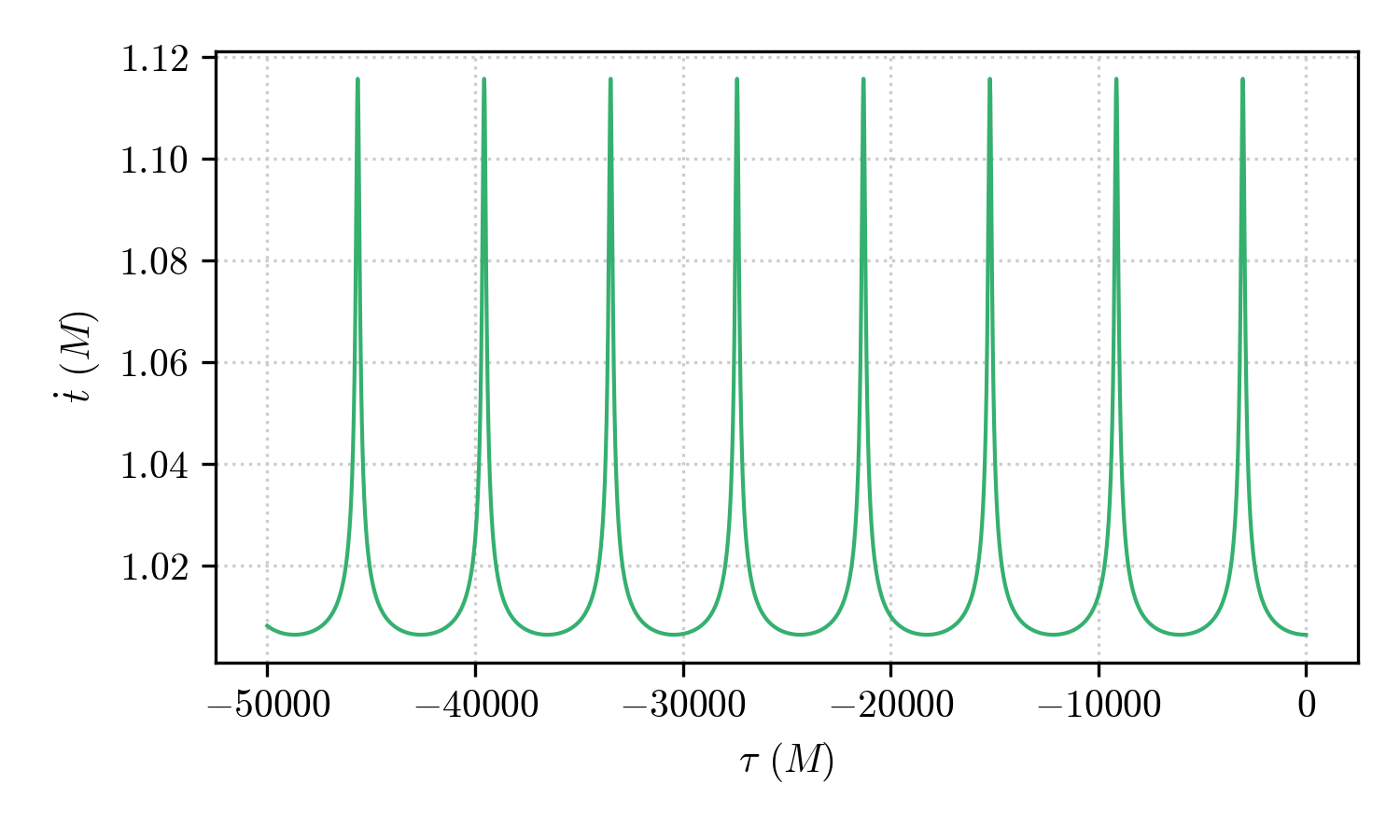
which clearly shows the Einstein delay (combination of gravitational redshift and Lorentz time-dilation) experienced by the orbit as it gets nearer of farther from the black hole.

Another possibility is to use the transform() of the Metric object (which is available only if transform_functions have been passed when the metric has been initialized, see Define your own space-time). This fuction acts on the integrated components of the geodesic and applies the transformation defined in the transform_functions, returning the an array of transformed values.

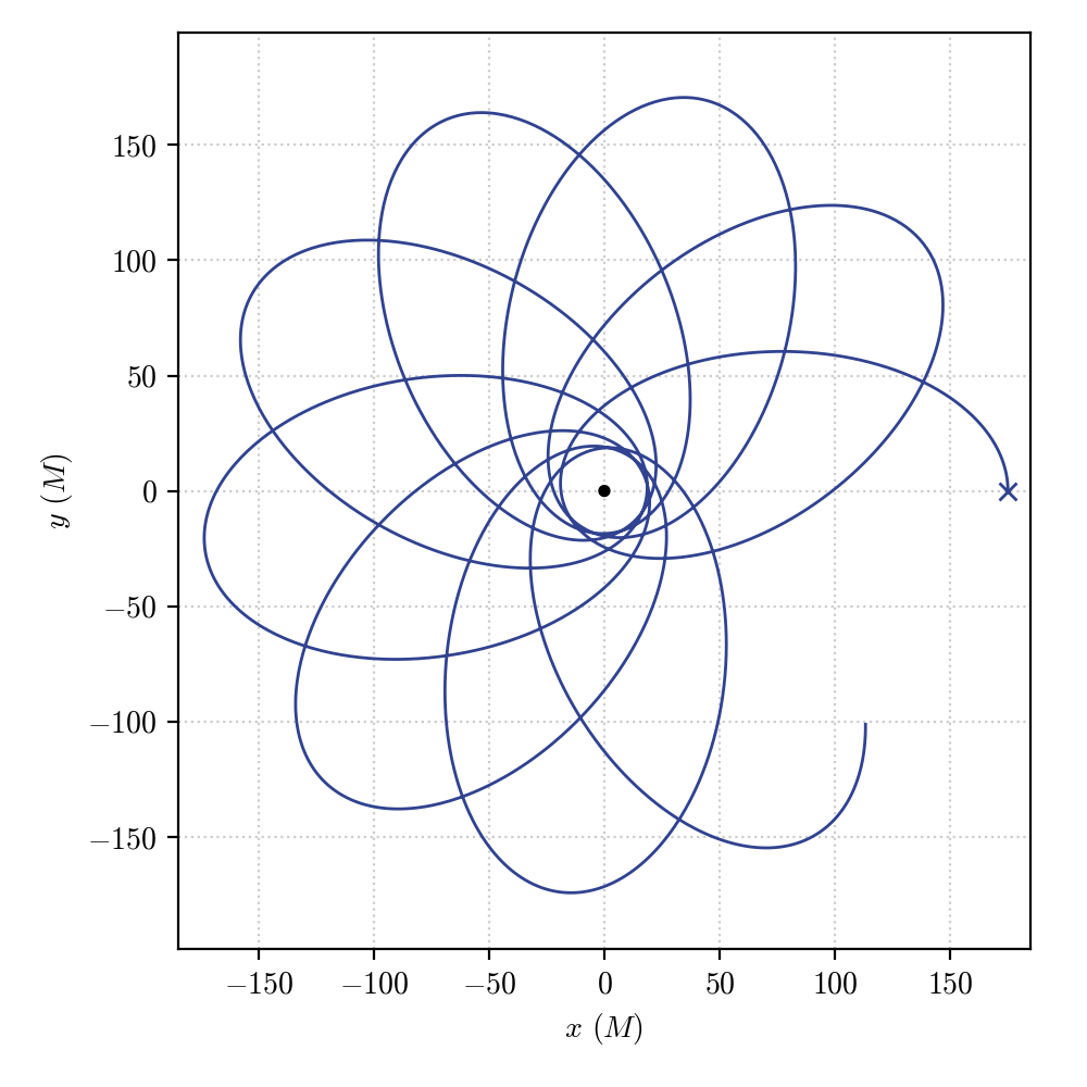
Having defined transformations to a pseudo-cartesian coordiante system (i.e. treating the Schwarzschild components as if they were actual spherical coordinates) one can transform the integrated geodesic by passing the transposed geo.x array, which is a \(4\times N\) array, to the transform() method

t, x, y, z = metric.transform(geo.x.T)

which one can directly plot

fig, ax = plt.subplots()

ax.plot(x, y)

# adding the central black hole

theta = np.linspace(0, 2*np.pi, 150)
x_bh = 2*np.cos(theta)
y_bh = 2*np.sin(theta)

ax.fill(x_bh, y_bh, color = "k")

obtaining a nice representation of the orbit:

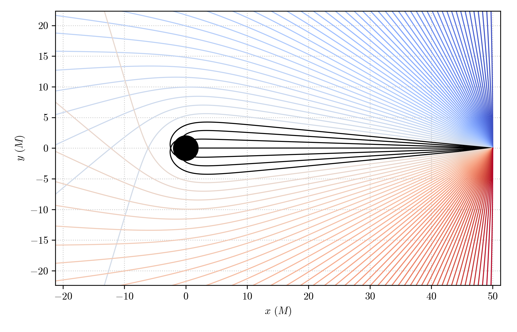
Of course, one can do the same with photons (null geodesics) and obtain a representation of a bundle of geodesics fired by an observer towards the black hole, assigning a color to the conditionally, given the exit state of the geodesic

import matplotlib as mpl
import matplotlib.pylot as plt

# Computing geodesics

phi_arr = np.linspace(-np.pi/2, np.pi/2, 101)

observer = pygro.Observer(metric, [0, 50, np.pi/2, 0], coframe = ["sqrt(A(r))*dt", "-dr/sqrt(A(r))", "-r*sin(theta)*dphi", "-r*dtheta"])

geo_arr = []

for phi in phi_arr:
    geo = pygro.Geodesic("null", geo_engine, verbose = False)
    geo.initial_x = observer.x
    geo.initial_u = observer.from_f1(0, phi, type = geo.type)

    geo_engine.integrate(geo, 1000, 1, verbose = False)

    geo_arr.append(geo)

# Plotting result

fig, ax = plt.subplots(figsize = (7, 4.5))

cmap = plt.get_cmap('coolwarm')
norm = mpl.colors.Normalize(vmin=-np.pi/2, vmax=np.pi/2)
mappable = mpl.cm.ScalarMappable(norm=norm, cmap=cmap)

for geo, phi in zip(geo_arr, phi_arr):
    t, x, y, z = metric.transform(geo.x.T)
    ax.plot(x, y, color = mappable.to_rgba(phi) if geo.exit != "horizon" else "k", linewidth = 1) # Color is assigned conditionally depending on wheter the geodesic hit the horizon

# Adding the black hole

theta = np.linspace(0, 2*np.pi, 150)
x_bh = 2*np.cos(theta)
y_bh = 2*np.sin(theta)

ax.fill(x_bh, y_bh, color = "k")

ax.set_xlabel(r'$x$ ($M$)')
ax.set_ylabel(r'$y$ ($M$)')

which gives out the following representation