Null geodesic integration

Null geodesics describe in General Relativity the space-time trajectory of massless particles (e.g. photons). Numerically integrating the equations of motions describing the dynamics of these particles allows performing ray-tracing, i.e. to reconstruct the paths that light-rays would follow on a curved space-time around a massive object.

In this tutorial we will examine the procedure in PyGRO to perform this operation and obtain the numerically integrated trajectory of a photon (or a bunch of them) in space-time.

Let’s assume that we have a Metric object appropriately initialized following the Define your own space-time tutorial and thus representing the Schwarzschild metric. Moreover, we assume that the we have initialized a GeodesicEngine object and linked it to the Schwarzschild metric, as done in the Integrate a geodesic in PyGRO tutorial. This also means that we have set a StoppingCriterion to stop the integration if a geodesic goes very close to the event horizon of the metric (resulting in a Geodesic.exit = "horizon" exit).

Now we can initialize a new null Geodesic in this set-up by simply defining a new object

geo = pygro.Geodesic("null", geo_engine)

Before being able to integrate the geodesic, we have to fix an initial position and 4-velocity for the geodesic. These quantities are stored in the Geodesic.initial_x and Geodesic.initial_u properties, respectively. While we can fix these properties by hand, it is more convenient to do so using the helper functions of the Geodesic class, that guarantee the normalization constraint imposed by the geodesic type.

We can hence use:

geo.set_starting_point(0, 50, np.pi/2, 0)
geo.set_starting_4velocity(u1 = -1, u2 = 0, u3 = 0.01)

to fix the initial position of the geodesic at a distance \(r=50M\) from the black hole, on the equatorial plane (\(\theta = \pi/2\)) and, without loss of generality at a coordinate time \(t=0\) and along the line \(\phi = 0\). Using the set_starting_4velocity() method, we have fixed an initial 4-velocity starting from its components \(u_r=-1\), \(u_\theta=0\) and \(u_\phi=0.01\), and we are letting the internal helper function of the Geodesic autonomously retrieve the corresponding value of \(u_t\) that satisfies the normalization condition at the given initial point.

We will be alerted of the successful initialization of the Geodesic object by the output:

>>> (PyGRO) INFO: Setting starting point
>>> (PyGRO) INFO: Setting initial 4-velocity.

Now we are ready to carry out the integration of the Geodesic following the scheme depicted in Integrate a geodesic in PyGRO.

Hence, we can call the method:

geo_engine.integrate(geo, 50, 1, verbose=True, accuracy_goal = 11, precision_goal = 11)

to integrate the Geodesic object geo up to a value of the affine parameter \(\tau = 50\), starting with an initial step of 1. The verbose = True keyword argument makes the integration verbose which will alert us of the status of the integration. We have also used specific precisiona and accuracy tolerances, for which we suggest reading the Integrators tutorial. In this case, we will be logged

>>> (PyGRO) INFO: Starting integration.
>>> (PyGRO) INFO: Integration completed in 0.038264 s with result 'done'.

signaling that the integration has been succesful, and has not met any horizon or stopping criterion (since it has an exit string 'done').

We can visualize the resulting geodesic following the Visualize the results tutorial:

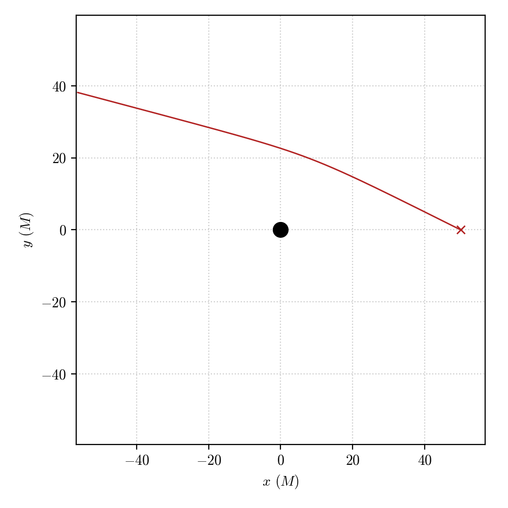
The geodesic obtained by the integration propagates in the gravitational field of the Schwarzschild black hole and gets deflected by a small angle as it approaches the central object.

We can try and repeat the integration by changing the initial 4-velocity, reducing its \(\theta\) component (e.g. by a factor 5) and making it plunge into the horizon.

geo_2 = pygro.Geodesic("null", geo_engine, verbose = True)
geo_2.set_starting_point(0, 50, np.pi/2, 0)
geo_2.set_starting_4velocity(u1 = -1, u2 = 0, u3 = 0.002)
geo_engine.integrate(geo_2, 100, 1)

resulting in

(PyGRO) INFO: Integration completed in 0.10361 s with result 'horizon'.

which can be visualized as

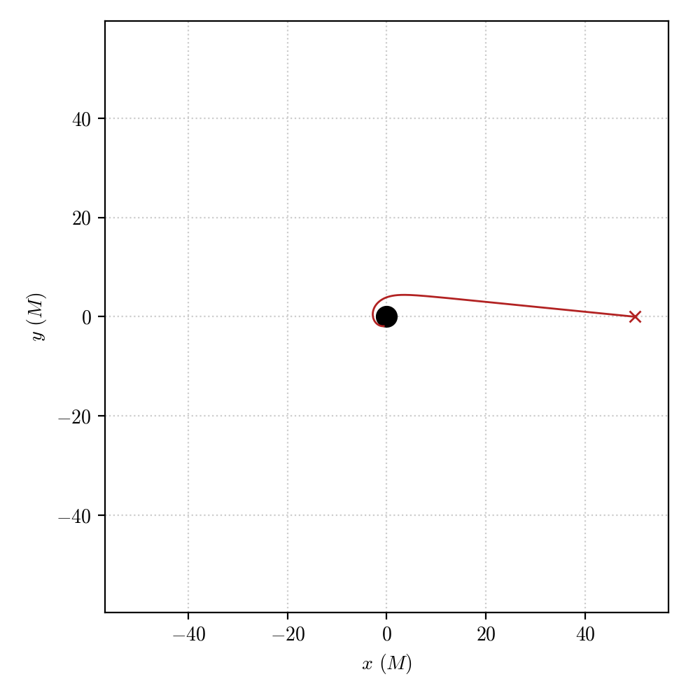
We can play around by changing the starting point of the geodesic and its 4-velocity to see how the the integrated geodesic changes depending on the initial data. Nevertheless, directly using the set_starting_4velocity() to fix the initial components of the 4-velocity has its drawebacks as one directly fixes the derivatives of the space-time coordinates at the initial time which in principle have no physical meaning. A much more physical way of fixing the initial conditions is to choose a physical observer, using the Observer class and use it to fix initial conditions for null geodesics starting from a specific direction in the observer’s reference frame.

This will be explained in more details in the Define a space-time Observer tutorial.